Technology focus: MIBI-TOF

This notebook will present a rough overview of the plotting functionalities that spatialdata implements for Visium data.

Loading the data

Please download the data from here: MIBI-TOF dataset and adjust the variable containing the location of the .zarr file.

mibitof_zarr_path = "./mibitof.zarr"

import spatialdata as sd

mibitof_sdata = sd.read_zarr(mibitof_zarr_path)
mibitof_sdata

SpatialData object with:
├── Images
│     ├── 'point8_image': SpatialImage[cyx] (3, 1024, 1024)
│     ├── 'point16_image': SpatialImage[cyx] (3, 1024, 1024)
│     └── 'point23_image': SpatialImage[cyx] (3, 1024, 1024)
├── Labels
│     ├── 'point8_labels': SpatialImage[yx] (1024, 1024)
│     ├── 'point16_labels': SpatialImage[yx] (1024, 1024)
│     └── 'point23_labels': SpatialImage[yx] (1024, 1024)
└── Table
      └── AnnData object with n_obs × n_vars = 3309 × 36
    obs: 'row_num', 'point', 'cell_id', 'X1', 'center_rowcoord', 'center_colcoord', 'cell_size', 'category', 'donor', 'Cluster', 'batch', 'library_id'
    uns: 'spatialdata_attrs'
    obsm: 'X_scanorama', 'X_umap', 'spatial': AnnData (3309, 36)
with coordinate systems:
▸ 'point8', with elements:
        point8_image (Images), point8_labels (Labels)
▸ 'point16', with elements:
        point16_image (Images), point16_labels (Labels)
▸ 'point23', with elements:
        point23_image (Images), point23_labels (Labels)

Visualise the data

We’re going to create a naiive visualisation of the data, overlaying the segmented cells and the tissue images. For this, we need to load the spatialdata_plot library which extends the sd.SpatialData object with the .pl module.

import spatialdata_plot

mibitof_sdata.pl.render_images().pl.render_labels().pl.show()

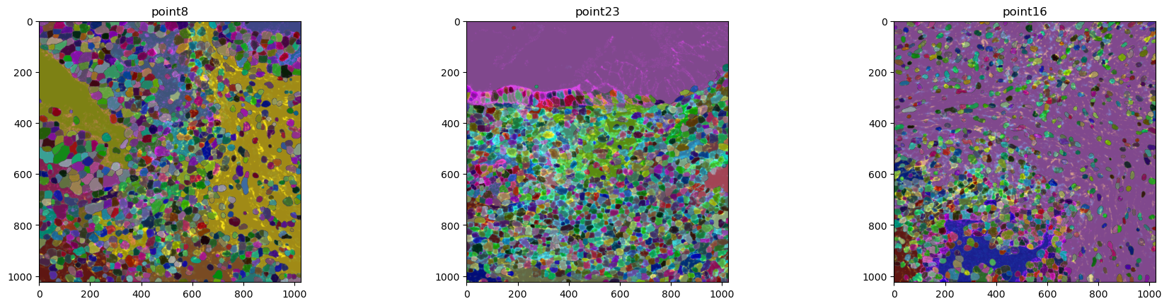
We can see that the data contains three coordinate systems (point8, point16 and point23) with image and cell segmentation information each. When giving no further parameters, one panel is generated per coordinate system with the members that have been specified in the function call. While it is hard to see, the cell labels overlay the tissue image nicely. To better show this, we will plot the data on individual ax objects.

import matplotlib.pyplot as plt

fig, axs = plt.subplots(ncols=3, nrows=1, figsize=(10, 4))

mibitof_sdata_subset = mibitof_sdata.pp.get_elements("point8")

mibitof_sdata_subset.pl.render_images().pl.show(ax=axs[0], title="image")

mibitof_sdata_subset.pl.render_labels().pl.show(ax=axs[1], title="labels")

mibitof_sdata_subset.pl.render_images().pl.render_labels().pl.show(ax=axs[2], title="both")

plt.tight_layout()

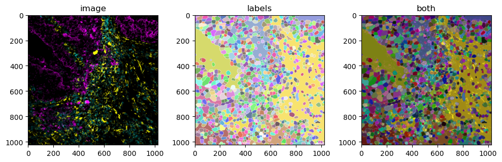
However, the segmentation masks are all shown in random colors since we have not provided any information on what they should encode. Such information can be found in the Table attribute (which is an anndata.AnnData table) of the SpatialData object,either in the data itself or the obs attribute.

mibitof_sdata["table"].to_df().head(3)

	ASCT2	ATP5A	CD11c	CD14	CD3	CD31	CD36	CD39	CD4	CD45	...	NRF2p	NaKATPase	PD1	PKM2	S6p	SDHA	SMA	VDAC1	XBP1	vimentin
9376-1	-0.099024	0.047260	-0.076592	-0.160894	-0.094239	-0.059072	-0.048790	-0.080359	-0.181162	-0.177686	...	-0.063972	-0.062695	-0.078785	-0.189159	-0.233837	0.038624	-0.502865	-0.016736	0.055549	-0.410221
9377-1	-0.081413	0.025841	-0.062929	0.071132	-0.086687	-0.072516	0.209030	0.067253	0.088813	-0.164108	...	0.116562	0.115541	-0.075863	0.024126	-0.318994	-0.043148	-0.120517	-0.058352	-0.197411	-0.179946
9378-1	-0.100959	-0.203419	-0.055992	-0.134076	-0.066981	-0.047282	-0.044181	-0.170404	-0.045016	-0.110186	...	-0.031722	-0.109969	-0.060554	-0.244716	-0.218434	-0.172760	-0.301259	-0.210778	0.042039	-0.266521

3 rows × 36 columns

mibitof_sdata["table"].obs.head(3)

	row_num	point	cell_id	X1	center_rowcoord	center_colcoord	cell_size	category	donor	Cluster	batch	library_id
9376-1	9479	8	2	65222.0	37.0	6.0	474.0	carcinoma	90de	Epithelial	1	point8_labels
9377-1	9480	8	4	65224.0	314.0	3.0	126.0	carcinoma	90de	Epithelial	1	point8_labels
9378-1	9481	8	5	65225.0	407.0	6.0	398.0	carcinoma	90de	Epithelial	1	point8_labels

Color the segmentation masks by a categorical variable

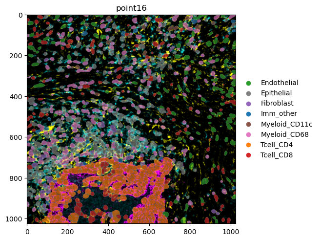
To use this information in our plot, we provide the column-name to be used for the color-enocoding to color in render_labels(). Here, spatialdata-plot automatically differentiates between categorical and numerical columns. Furthermore, we subset the data to only one coordinate system.

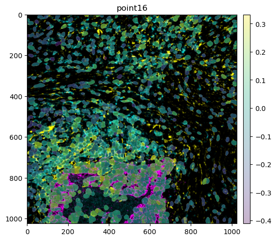
mibitof_sdata.pp.get_elements("point16").pl.render_images().pl.render_labels(color="Cluster").pl.show()

mibitof_sdata.pp.get_elements("point16").pl.render_images().pl.render_labels(color="ASCT2").pl.show()