Integrate/aggregate signals across spatial layers

In this notebook, we will describe some usage principles for the aggregate method.

Let’s first import some useful libraries and create some dummy data to show the example.

%load_ext autoreload
%autoreload 2

%load_ext jupyter_black

import os

os.environ["USE_PYGEOS"] = "0"

import spatialdata_plot
from spatialdata.datasets import blobs

sdata = blobs()
sdata

SpatialData object with:
├── Images
│     ├── 'blobs_image': SpatialImage[cyx] (3, 512, 512)
│     └── 'blobs_multiscale_image': MultiscaleSpatialImage[cyx] (3, 512, 512), (3, 256, 256), (3, 128, 128)
├── Labels
│     ├── 'blobs_labels': SpatialImage[yx] (512, 512)
│     └── 'blobs_multiscale_labels': MultiscaleSpatialImage[yx] (512, 512), (256, 256), (128, 128)
├── Points
│     └── 'blobs_points': DataFrame with shape: (<Delayed>, 4) (2D points)
├── Shapes
│     ├── 'blobs_circles': GeoDataFrame shape: (5, 2) (2D shapes)
│     ├── 'blobs_multipolygons': GeoDataFrame shape: (2, 1) (2D shapes)
│     └── 'blobs_polygons': GeoDataFrame shape: (5, 1) (2D shapes)
└── Tables
      └── 'table': AnnData (26, 3)
with coordinate systems:
▸ 'global', with elements:
        blobs_image (Images), blobs_multiscale_image (Images), blobs_labels (Labels), blobs_multiscale_labels (Labels), blobs_points (Points), blobs_circles (Shapes), blobs_multipolygons (Shapes), blobs_polygons (Shapes)

import matplotlib.pyplot as plt

fig, axs = plt.subplots(ncols=3, figsize=(12, 3))

sdata.pl.render_images("blobs_image").pl.show(ax=axs[0])
sdata.pl.render_labels("blobs_labels").pl.show(ax=axs[1])
sdata.pl.render_points("blobs_points").pl.show(ax=axs[2])

We can do various type of aggregations:

• aggregate images by labels

• aggregate points by shapes

• aggregate shapes by shapes

Aggregations between mixed raster and non-raster types are currently not supported (but will be).

The API function for aggregation is spatialdata.aggregate. It is also possible to perform aggregation using the convenience method spatialdata.SpatialData.aggregate, which simply calls the previous one and automatically fills some values (values_sdata and by_sdata) with self; we will see this below.

Let’s start with aggregation of images by labels. This can be achieved with one line of code:

Aggregating images by labels

sdata_im = sdata.aggregate(values="blobs_image", by="blobs_labels", agg_func="mean")

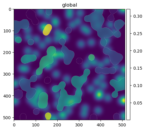
As default, the aggregation function is sum but it can be changed with the agg_func parameter. We can inspect the table inside the returned SpatialData object to confirm that the operation results in retrieving the mean intensity of each image channel within the boundaries of the labels. We can also visualize the results with spatialdata-plot. By overlaying the labels with the channel where we performed aggregation, we can better appreciate the results. Labels that overlap with high intensity of the channels have indeed a higher mean intensity.

The features of the new table are the following:

sdata_im["table"].var_names

Index(['channel_0_mean', 'channel_1_mean', 'channel_2_mean'], dtype='object')

ax = plt.gca()
sdata.pl.render_images("blobs_image", cmap="viridis", channel=1).pl.show(ax=ax)
sdata_im.pl.render_labels(color="channel_1_mean", fill_alpha=0.5).pl.show(ax=ax)

We can also aggregate points by shapes. For example, let’s count the number of points that overlap each shape.

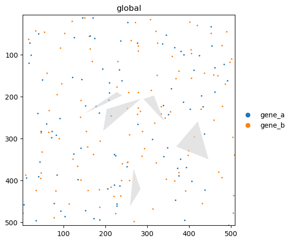
Here we see the points and shapes that we will use for aggregation.

Aggregating points by shapes

sdata["blobs_points"].compute()

	x	y	genes	instance_id
0	46	395	gene_b	9
1	334	224	gene_b	7
2	221	438	gene_b	3
3	44	356	gene_a	9
4	103	49	gene_b	4
...	...	...	...	...
195	381	92	gene_a	8
196	188	306	gene_b	5
197	368	447	gene_a	7
198	23	101	gene_a	6
199	144	159	gene_a	6

200 rows × 4 columns

sdata.pl.render_points(color="genes").pl.render_shapes("blobs_polygons", fill_alpha=0.6).pl.show()

The value_key parameters specifies which columns of the points dataframe will be aggregated.

sdata_shapes = sdata.aggregate(values="blobs_points", by="blobs_polygons", value_key="genes", agg_func="count")
sdata_shapes

SpatialData object with:
├── Shapes
│     └── 'blobs_polygons': GeoDataFrame shape: (5, 1) (2D shapes)
└── Tables
      └── 'table': AnnData (5, 2)
with coordinate systems:
▸ 'global', with elements:
        blobs_polygons (Shapes)

Let’s color by the var value gene_b of the aggregate table (that is, we color by the numbers of points of type gene_b inside each shape).

ax = plt.gca()
sdata.pl.render_points(color="genes").pl.show(ax=ax)
sdata_shapes.pl.render_shapes(color="gene_b", fill_alpha=0.7).pl.show(ax=ax)

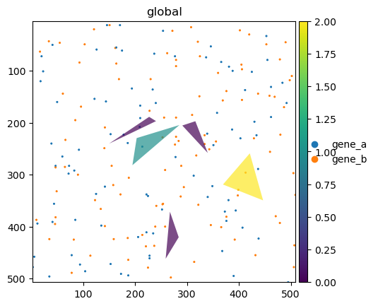
The colormap represents the number of counts for the selected variable (gene “b”). The rightmost polygon has correctly a value of 2, as there are 2 transcripts (points) of type “b” overlapping the polygon area.

Aggregating shapes by shapes, and information from different locations

In this example let’s show four things:

• aggregating shapes by shapes

• aggregating layers from different SpatialData objects

• aggregating signals from different location within the same SpatialData object (value_key parameter).

• explain the difference of the aggregate() function and the aggregate() method

To do so, let’s create two SpatialData objects:

• one with the blobs_circles geometries, but adding some extra annotations, both as new GeoDataFrame columns, and in an AnnData table;

• one wiht two large rectangles that we will use to aggregate the circles by.

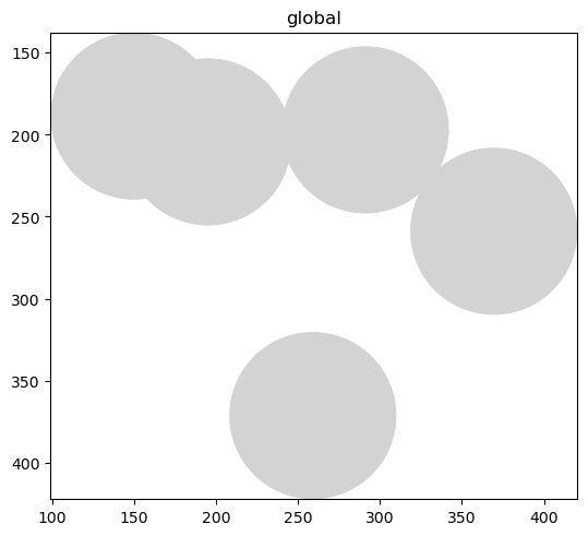
Creating the circles object

sdata.pl.render_shapes("blobs_circles").pl.show()

import numpy as np
import pandas as pd
from anndata import AnnData
from numpy.random import default_rng
from spatialdata import SpatialData
from spatialdata.models import TableModel

RNG = default_rng(42)

adata_circles = AnnData(
    RNG.normal(size=(5, 3)),
    var=pd.DataFrame(index=["gene_h", "gene_k", "gene_l"]),
    obs=pd.DataFrame(
        {
            "categorical": ["a", "a", "b", "c", "d"],
            "region": "blobs_circles",
            "instance_id": np.arange(5),
        }
    ),
)
adata_circles.obs["categorical"] = adata_circles.obs["categorical"].astype("category")
adata_circles.obs["region"] = adata_circles.obs["region"].astype("category")
adata_circles = TableModel.parse(adata_circles, region="blobs_circles", region_key="region", instance_key="instance_id")
sdata_circles = SpatialData(shapes={"blobs_circles": sdata["blobs_circles"]}, tables={"table": adata_circles})

# let's add two numerical columns to the GeoDataFrame
sdata_circles["blobs_circles"]["feature_m"] = RNG.normal(size=(5))
sdata_circles["blobs_circles"]["feature_n"] = RNG.normal(size=(5))

import matplotlib.pyplot as plt

fig, axs = plt.subplots(ncols=3, figsize=(12, 3))
sdata_circles.pl.render_shapes(color="gene_h").pl.show(ax=axs[0], title="gene_h")
sdata_circles.pl.render_shapes(color="feature_m").pl.show(ax=axs[1], title="feature_m")
sdata_circles.pl.render_shapes(color="categorical").pl.show(ax=axs[2], title="categorical")

Creating the squares object

import geopandas as gpd
from shapely import linearrings, polygons
from spatialdata.models import ShapesModel


def _make_squares(centroid_coordinates: np.ndarray, half_widths: list[float]) -> polygons:
    linear_rings = []
    for centroid, half_width in zip(centroid_coordinates, half_widths):
        min_coords = centroid - half_width
        max_coords = centroid + half_width

        linear_rings.append(
            linearrings(
                [
                    [min_coords[0], min_coords[1]],
                    [min_coords[0], max_coords[1]],
                    [max_coords[0], max_coords[1]],
                    [max_coords[0], min_coords[1]],
                ]
            )
        )
    s = polygons(linear_rings)
    polygon_series = gpd.GeoSeries(s)
    cell_polygon_table = gpd.GeoDataFrame(geometry=polygon_series)
    return ShapesModel.parse(cell_polygon_table)


sdata_squares = SpatialData(
    shapes={"squares": _make_squares(np.atleast_2d([[100, 200], [400, 200]]), half_widths=[100, 80])}
)

ax = plt.gca()

sdata_squares.pl.render_shapes("squares", na_color="red", alpha=0.5).pl.show(ax=ax)
sdata_circles.pl.render_shapes("blobs_circles", alpha=0.5).pl.show(ax=ax)

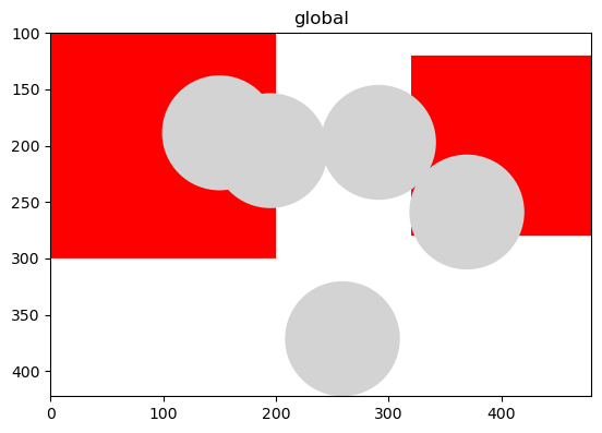
We will now aggregate the various quantities. Notice how the value_key can be used to aggregate values that are located in different places in the SpatialData object:

1. matrix X of the AnnData table (names given by .var_names);

2. .obs DataFrame of the AnnData table;

3. columns of the GeoDataFrame.

Notice also that the API deal both with numerical and categorical values, and can aggregate multiple numerical columns at the same time.

Case: value_key referring to var_names

from spatialdata import aggregate

sdata_gene_exp = aggregate(
    values_sdata=sdata_circles,
    by_sdata=sdata_squares,
    values="blobs_circles",
    by="squares",
    value_key=["gene_h", "gene_k"],
    table_name="table",
)
print(sdata_gene_exp)
print()
print(sdata_gene_exp["table"].var_names)

SpatialData object with:
├── Shapes
│     └── 'squares': GeoDataFrame shape: (2, 1) (2D shapes)
└── Tables
      └── 'table': AnnData (2, 2)
with coordinate systems:
▸ 'global', with elements:
        squares (Shapes)

Index(['gene_h', 'gene_k'], dtype='object')

Case: value_key referring to GeoDataFrame columns

sdata_feature = aggregate(
    values_sdata=sdata_circles,
    by_sdata=sdata_squares,
    values="blobs_circles",
    by="squares",
    value_key="feature_m",
)
print(sdata_feature)
print()
print(sdata_feature["table"].var_names)

SpatialData object with:
├── Shapes
│     └── 'squares': GeoDataFrame shape: (2, 1) (2D shapes)
└── Tables
      └── 'table': AnnData (2, 1)
with coordinate systems:
▸ 'global', with elements:
        squares (Shapes)

Index(['feature_m'], dtype='object')

Case: value_key referring to obs columns

sdata_categorical = aggregate(
    values_sdata=sdata_circles,
    by_sdata=sdata_squares,
    values="blobs_circles",
    by="squares",
    value_key="categorical",
)
print(sdata_categorical)
print()
print(sdata_categorical["table"].var_names)

SpatialData object with:
├── Shapes
│     └── 'squares': GeoDataFrame shape: (2, 1) (2D shapes)
└── Tables
      └── 'table': AnnData (2, 4)
with coordinate systems:
▸ 'global', with elements:
        squares (Shapes)

Index(['a', 'b', 'c', 'd'], dtype='object')

import matplotlib.pyplot as plt

fig, axs = plt.subplots(ncols=3, figsize=(12, 3))

sdata_gene_exp.pl.render_shapes("squares", color="gene_h", alpha=0.5).pl.show(ax=axs[0], title="gene_h")

sdata_feature.pl.render_shapes("squares", color="feature_m", alpha=0.5).pl.show(ax=axs[1], title="feature_m")

sdata_categorical.pl.render_shapes("squares", color="a", alpha=0.5).pl.show(ax=axs[2], title="categorical")
sdata_circles.pl.render_shapes(color="categorical").pl.show(ax=axs[2], title="categorical")

The method vs the function

Above we used the aggregate() function. The method version is equivalent and it is a convenience function that simply fills in eventually missing values of values_sdata and by_sdata with self.

So these two functions are equivalent:

res0 = aggregate(
    values_sdata=sdata_circles,
    by_sdata=sdata_squares,
    values="blobs_circles",
    by="squares",
    value_key="feature_m",
)

res1 = sdata_circles.aggregate(
    by_sdata=sdata_squares,
    values="blobs_circles",
    by="squares",
    value_key="feature_m",
)

One can also directly pass to values or by a SpatialElement. So also this is an equivalent call, except for the fact that now the string squares is never passed to aggregate(), so it will be used a default name for the name of the SpatialElement

res2 = sdata_circles.aggregate(
    by=sdata_squares["squares"],
    values="blobs_circles",
    value_key="feature_m",
)

from anndata.tests.helpers import assert_equal

assert_equal(res0["table"], res1["table"])
assert_equal(res0["table"].X, res2["table"].X)

res0["table"].obs

	instance_id	region
0	0	squares
1	1	squares

res2["table"].obs

	instance_id	region
0	0	by
1	1	by