Working with annotations in SpatialData

Introduction

The spatialdata framework supports both the representation of SpatialElements (images, labels, points, shapes) and of annotations for these elements. As we will explore in this notebook, some types of SpatialElements can contain some annotatoins within themselves, but the general approach we take is to represent SpatialElements and annotations in separate objects, which allows or more granular control and composability.

For storing annotations we rely on the AnnData data structure, and we refer to this object also with the term table.

In this notebook we will show the following:

• Introduction
• Store annotations in a SpatialElement
   • Labels
   • Shapes (circles, polygons/multipolygons)
   • Points
   • Images
• Store annotations with AnnData tables
   • Table metadata (annotation targets)
   • Retrieving annotations with get_values()
     • Where to store the annotation
• Operations on tables
   • Find which elements a table is annotating
   • Change the annotation target of table
   • Construct a table annotating 0 SpatialElements
   • Construct a table annotating 1 or more SpatialElements
• Performing SQL like joins
   • A note on joins
• A use case for table

Store annotations in a SpatialElement

We will consider an example datasets, blobs, which contains a copy for each type of SpatialElement we support.

from spatialdata.datasets import blobs

sdata = blobs()
sdata

SpatialData object with:
├── Images
│     ├── 'blobs_image': SpatialImage[cyx] (3, 512, 512)
│     └── 'blobs_multiscale_image': MultiscaleSpatialImage[cyx] (3, 512, 512), (3, 256, 256), (3, 128, 128)
├── Labels
│     ├── 'blobs_labels': SpatialImage[yx] (512, 512)
│     └── 'blobs_multiscale_labels': MultiscaleSpatialImage[yx] (512, 512), (256, 256), (128, 128)
├── Points
│     └── 'blobs_points': DataFrame with shape: (<Delayed>, 4) (2D points)
├── Shapes
│     ├── 'blobs_circles': GeoDataFrame shape: (5, 2) (2D shapes)
│     ├── 'blobs_multipolygons': GeoDataFrame shape: (2, 1) (2D shapes)
│     └── 'blobs_polygons': GeoDataFrame shape: (5, 1) (2D shapes)
└── Tables
      └── 'table': AnnData (26, 3)
with coordinate systems:
▸ 'global', with elements:
        blobs_image (Images), blobs_multiscale_image (Images), blobs_labels (Labels), blobs_multiscale_labels (Labels), blobs_points (Points), blobs_circles (Shapes), blobs_multipolygons (Shapes), blobs_polygons (Shapes)

Labels

Labels object cannot contain annotations within themselves; instead, a table is needed for that. Let’s see how to compute their indices.

2D and 3D labels have respectively dimensions ('y', 'x') and ('z', 'y', 'x'). Given a labels object, the instances are defined by all the pixels whose value is equal to a particular index. In order to identify the indices one can therefore compute the unique values in the labels object (for a multiscale labels the largest resolution should be considered). This is conveniently done by the private function _get_unique_label_values_as_index(); in one of the next releases we will include this function as a special case of the get_values() function, discussed later in the notebook.

Here we show how to use this function to identify the indices of the instances encoded by the labels object, and also how to manually compute this information.

import numpy as np
from spatialdata._core.query.relational_query import _get_unique_label_values_as_index

print(_get_unique_label_values_as_index(sdata["blobs_multiscale_labels"]))
print(np.unique(sdata["blobs_multiscale_labels"]["scale0"]["image"].data.compute()))

Index([ 0,  1,  2,  3,  4,  5,  6,  8,  9, 10, 11, 12, 13, 15, 16, 17, 18, 19,
       20, 22, 23, 24, 25, 26, 27, 29, 30],
      dtype='int16')
[ 0  1  2  3  4  5  6  8  9 10 11 12 13 15 16 17 18 19 20 22 23 24 25 26
 27 29 30]

Shapes (circles, polygons/multipolygons)

Shapes are GeoDataFrame object, a subclass of GeoDataFrame where the geometric information is specified in the geometry column. Since they are dataframes, they in particular contain the index, which can be accessed with

sdata["blobs_multipolygons"].index

RangeIndex(start=0, stop=2, step=1)

Circles require a column named radius and the rows in the columns geometry need to be of type shapely.Point. Polygons/multipolygons require the type of the rows in the column geometry to be shapely.Polygon/shapely.MultiPolygon. These are the only requirements, and the extra columns can be used for annotation.

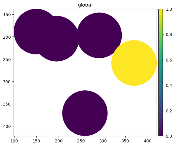
sdata["blobs_circles"]["my_value"] = [0, 0, 0, 0, 1]
sdata["blobs_circles"]

	geometry	radius	my_value
0	POINT (291.062 197.065)	51	0
1	POINT (259.026 371.319)	51	0
2	POINT (194.973 204.414)	51	0
3	POINT (149.926 188.623)	51	0
4	POINT (369.422 258.900)	51	1

import spatialdata_plot

sdata.pl.render_shapes("blobs_circles", color="my_value").pl.show()

Points

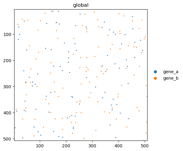
Points are represented as “lazy” (using Dask) pandas dataframes. Similarly as above, they have an index. The spatial information is specified by the x and y columns (for 2D points) and the x, y, z columns (for 3D points). The rest of the columns can be used to store annotations. The blobs dataset already stores some annotations in those columns.

sdata["blobs_points"].compute()

	x	y	genes	instance_id
0	46	395	gene_b	9
1	334	224	gene_b	7
2	221	438	gene_b	3
3	44	356	gene_a	9
4	103	49	gene_b	4
...	...	...	...	...
195	381	92	gene_a	8
196	188	306	gene_b	5
197	368	447	gene_a	7
198	23	101	gene_a	6
199	144	159	gene_a	6

200 rows × 4 columns

sdata.pl.render_points(color="genes").pl.show()

Images

2D and 3D images have respectively dimensions ('c', 'y', 'x') and ('c', 'z', 'y', 'x'). Unlike for the SpatialElements above, images do not contain information on instances and in particular they do not have an index. Nevertheless, the coordinates of the dimension c of images can be specified, thus giving a name for each channel.

Channels can be accessed using the utils function get_channels(), which operates on both single-scale and multi-scale images.

from spatialdata.models import get_channels

get_channels(sdata["blobs_multiscale_image"])

[0, 1, 2]

The channels can also be accessed directly from the xarray.DataArray object. For instance for a single-scale image we have

sdata["blobs_image"].c.values

array([0, 1, 2])

To set the channels we recommend to use the parsers Image2DModel.parse() and Image3DModel.parse(). For instance

from spatialdata.models import Image2DModel

sdata["blobs_image"] = Image2DModel.parse(sdata["blobs_image"], c_coords=["r", "g", "b"])
get_channels(sdata["blobs_image"])

['r', 'g', 'b']

Store annotations with AnnData tables

Tables can annotate any SpatialElement that have an index, so they can annotate labels, shapes and points. Tables can also be specified without defining the annotation target; images do not have an index so they cannot be annotated by a table, but one could use a table without an annotation target to effectively annotate the channels of the image. Tables cannot annotate tables.

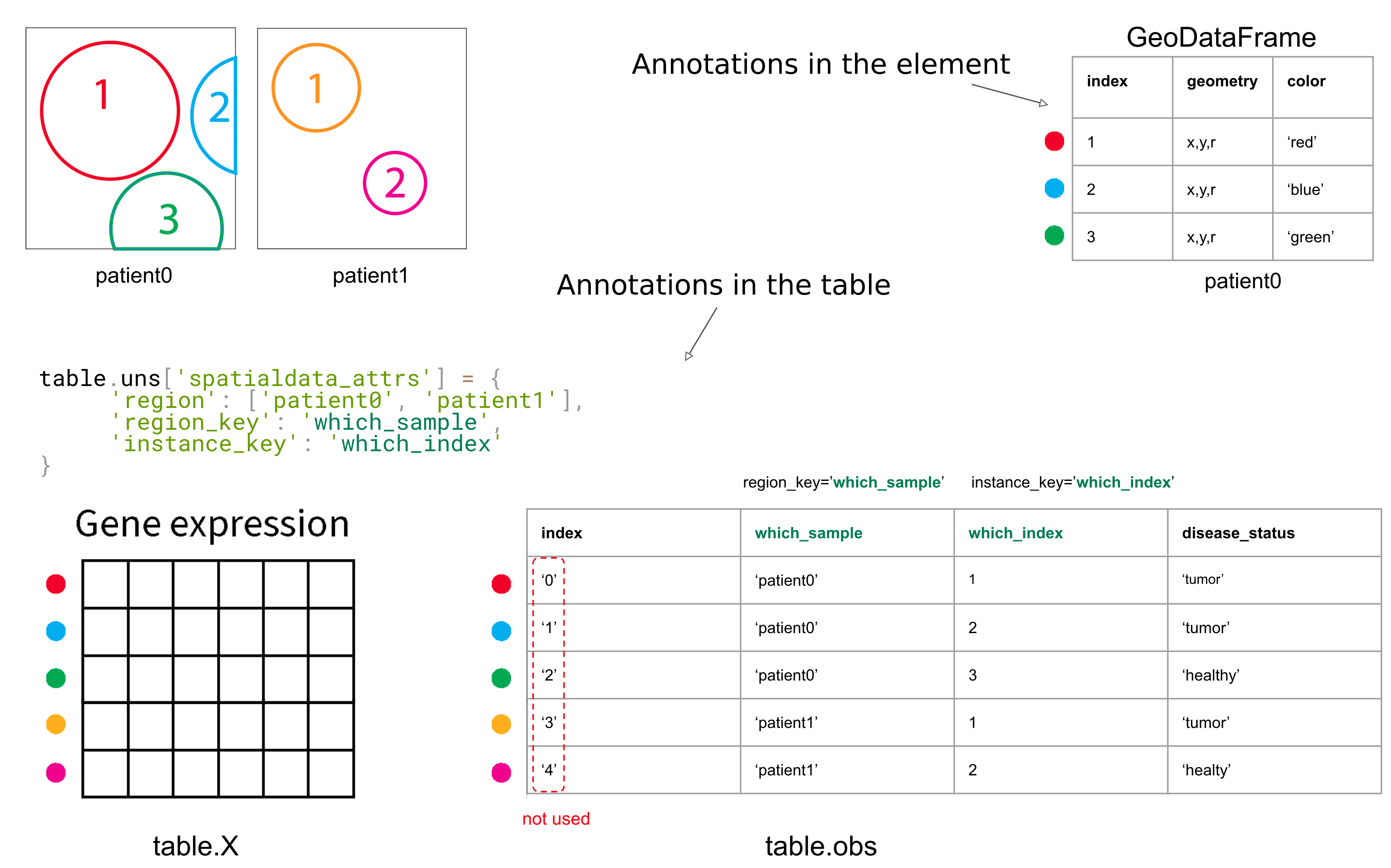
An AnnData table offers a more powerful way to store annotations as opposed to the methods described before. The AnnData object can store sparse and dense matrices, multiple layers (=variants) of these matrices, and can store annotations for the rows and columns for these matrices in terms of tensors, dataframes and matrices of pairwise relationships. We refer to the anndata documentation (https://anndata.readthedocs.io/en/latest/) for a full description of this and here we limit to the following graphical schematic.

Table metadata (annotation targets)

Each table contains some metadata that defines the annotation target (if any) of the table. This metadata is constituted by:

• the region, region_key and instance_key triplet, stored in table.uns;

• two columns of the DataFrame stored in table.obs.

A table that doesn’t annotate any element doesn’t contain any of the above metadata. Instead, in order to define the annotation targets of a table, the above metadata is defined as follows:

• region is either a string either a list of strings, and describes the list of targets, i.e. the SpatialElements that the table annotates.

• region_key is a string, and is the name of a column of the dataframe table.obs which describes, for each row, which is the SpatialElement that the rows refers to;

• instance_key is a string, and is the name of a column of the dataframe table.obs which describes, for each row, which is the index of the particular annotated instance (which is inside the SpatialElement annotated by the row).

A few more details on the two dataframe columns.

• The column named after region_key must have string either categorical type; it should nevertheless be categorical and the framework will warn the user to convert it as categorical before performing computationally expensive operations.

• The column named after instance_key must be either have numerical either string type.

Finally, you may notice that the information contained in region is redunant (as it can be computed as the list of unique values of the column named after region_key) and it may even get out-of-sync (for instance after subsetting the rows). For these reasons, in a future release we will simplify the metadata by dropping region, deriving it automatically instead. Anyway, currently we are maintaining it for legacy reasons.

Warning! Please note that we haven’t mentioned the index of the table. In fact, we do not use the index of the table!

The above information is summarized in the following graphical slide.

Retrieving annotations with get_values()

We provide a function get_values() that can be useful to retrive one or more columns of annotations for an element, independently if the annotations is stored in a table or in the elment. Here is an example.

sdata["blobs_points"].compute()

	x	y	genes	instance_id
0	46	395	gene_b	9
1	334	224	gene_b	7
2	221	438	gene_b	3
3	44	356	gene_a	9
4	103	49	gene_b	4
...	...	...	...	...
195	381	92	gene_a	8
196	188	306	gene_b	5
197	368	447	gene_a	7
198	23	101	gene_a	6
199	144	159	gene_a	6

200 rows × 4 columns

from spatialdata import get_values

get_values(value_key="genes", element=sdata["blobs_points"])

	genes
0	gene_b
1	gene_b
2	gene_b
3	gene_a
4	gene_b
...	...
195	gene_a
196	gene_b
197	gene_a
198	gene_a
199	gene_a

200 rows × 1 columns

sdata["table"].var_names

Index(['channel_0_sum', 'channel_1_sum', 'channel_2_sum'], dtype='object')

get_values(value_key="channel_0_sum", sdata=sdata, element_name="blobs_labels", table_name="table")

	channel_0_sum
instance_id
1	1309.369255
2	1535.995388
3	855.965478
4	614.497990
5	212.404587
6	482.633650
8	518.004680
9	258.186892
10	159.661750
11	3.438841
12	80.604196
13	155.678618
15	230.130425
16	150.663043
17	466.641687
18	2.271171
19	1.270513
20	118.423858
22	85.710077
23	285.418051
24	24.794733
25	220.373520
26	1.278647
27	113.662394
29	100.544497
30	59.460201

Where to store the annotation

Here are some recommendation on when to store the annotations in the SpatialElement and when in the AnnData table:

• we suggest to use the AnnData table when the annotations are complex, require the use of dense or sparse matrices and when there could be the need to reuse them between elements;

• for small annotations, like storing the name or some comments for some regions of interest sometimes elements annotation are more handy;

• when a point element is large (from 100 million rows), it may be worth, from a performance perspective, to store the annotation information directly in the point element instead that using an external AnnData table.

Operations on tables

Find which elements a table is annotating

Let’s now see an example. Blobs contains one table. Let’s see what it is annotating by looking at the region, region_key and instance_key metadata, which can be accessed using the utils function get_region_key().

from spatialdata.models import get_table_keys

region, region_key, instance_key = get_table_keys(sdata["table"])
print(region, region_key, instance_key)

blobs_labels region instance_id

We can see that this information is present in sdata["table"].obs. Here region are the names of the SpatialElements being annotated, the region_key corresponds to the column in .obs containing per row which SpatialElement is annotated by that row and instance_key specifies the column with per row the information which index of the SpatialElement the table is annotating.

sdata["table"].obs.head()

	instance_id	region
1	1	blobs_labels
2	2	blobs_labels
3	3	blobs_labels
4	4	blobs_labels
5	5	blobs_labels

If we want to retrieve either of the three, there are three helper functions that allow for this, namely get_annotated_regions, get_region_key_column and get_instance_key_column. Either of these take only the AnnDatatable as an argument. Below we show an example:

from spatialdata import SpatialData as sd

regions = sd.get_annotated_regions(sdata["table"])
print(regions)

blobs_labels

region_column = sd.get_region_key_column(sdata["table"])
print(region_column.head())

1    blobs_labels
2    blobs_labels
3    blobs_labels
4    blobs_labels
5    blobs_labels
Name: region, dtype: category
Categories (1, object): ['blobs_labels']

Change the annotation target of table

We have a helper function, set_table_annotates_spatialelement to change the metadata regarding the annotation target of table in a SpatialData object. This function takes as arguments the table_name, region and optionally the region_key and instance_key. The latter two don’t have to necessarily be specified if the table is already annotating a SpatialElement. The current values will be reused if not specified. For any of the arguments specified, they must be present at their respective location in the SpatialDataobject or table.

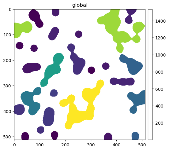
Here we will create a new circles element, with a circle for each instance of the labels element, and we will make the table annotate this new element. Let’s plot the labels with their annotations, let’s set the table to annotate the new element and then let’s also plot it.

sdata.table.var_names

Index(['channel_0_sum', 'channel_1_sum', 'channel_2_sum'], dtype='object')

sdata.pl.render_labels("blobs_labels", color="channel_0_sum", fill_alpha=1.0).pl.show()

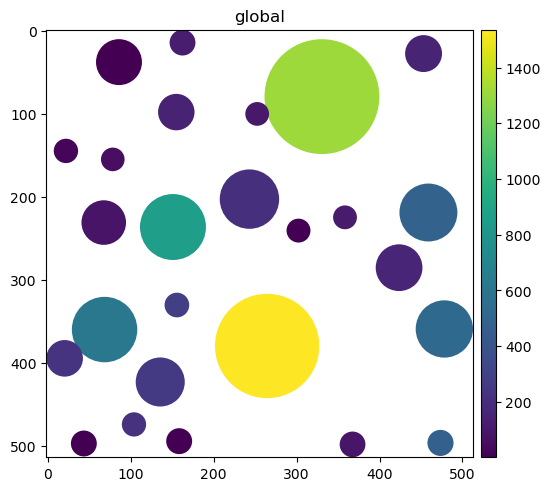
from spatialdata import to_circles

sdata["labels_as_circles"] = to_circles(sdata["blobs_labels"])

sdata["table"].obs["region"] = "labels_as_circles"
# no need to reassign the instance_key column 'instance_id' sicne the instances are the same as for labels
sdata.set_table_annotates_spatialelement("table", region="labels_as_circles")

sdata.pl.render_shapes("labels_as_circles", color="channel_0_sum").pl.show()

Construct a table annotating 0 SpatialElements

Tables in Spatialdata are AnnData tables. Creating a table that does not annotate a SpatialElement is as simple as constructing an Anndata table. In this case the table should not contain region, region_key and instance_key metadata. Here an example of a table storing a dummy codebook:

from anndata import AnnData
from spatialdata.models import TableModel

codebook_table = AnnData(obs={"Gene": ["Gene1", "Gene2", "Gene3"], "barcode": ["03210", "23013", "30121"]})

# We don't specify arguments related to metadata as we don't annotate a SpatialElement.
sdata_table = TableModel.parse(codebook_table)
sdata["codebook"] = sdata_table
sdata["codebook"].obs

	Gene	barcode
0	Gene1	03210
1	Gene2	23013
2	Gene3	30121

Construct a table annotating 1 or more SpatialElements

Now let us create a table that annotates multiple SpatialElements. Note that the order of the indices does not have to match the order of the indices in the SpatialElement. To showcase this we perform a permutation of the indices. Also, the dtypeof the index column of the SpatialElement must match the dtype of the instance_key column in the table. If this is not the case this will result in an error when trying to add the table to the SpatialData object. Lastly, not every index of the SpatialElement has to be present in the instance_key column of the SpatialData table and vice versa. We will later show functions to deal with these cases.

polygon_index = list(sdata.shapes["blobs_polygons"].index)
# We have to do a compute here as points are lazily loaded using dask.
point_index = list(sdata["blobs_points"].index.compute())

region_column = ["blobs_polygons"] * len(polygon_index) + ["blobs_points"] * len(point_index)
instance_id_column = polygon_index + point_index

import numpy as np

RNG = np.random.default_rng()
table = AnnData(
    X=np.zeros((len(region_column), 1)),
    obs={"region": region_column, "instance_id": instance_id_column},
)
table = table[RNG.permutation(table.obs.index), :].copy()

# Now we have to specify all 3 annotation metadata fields.
sdata_table = TableModel.parse(
    table, region=["blobs_polygons", "blobs_points"], region_key="region", instance_key="instance_id"
)

# When adding the table now, it is validated for presence of annotation targets in the sdata object.
sdata["annotations"] = sdata_table

Performing SQL like joins

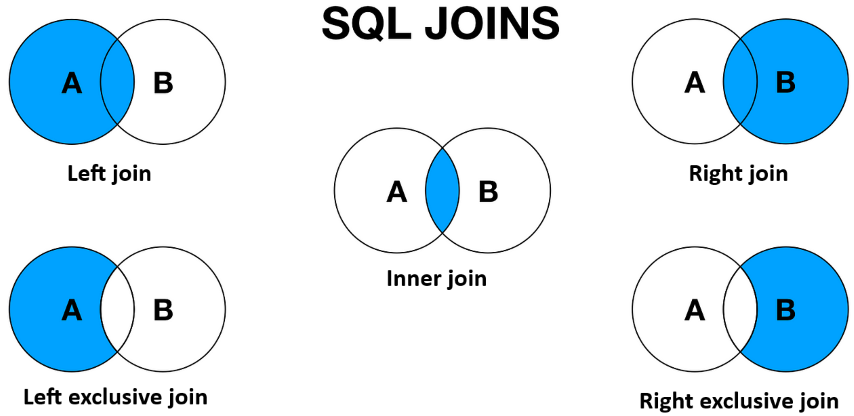
In order to retrieve matching and non-matching parts of a SpatialElement and the annotating tables we can perform SQL like join operations on the table. For this, we have the function join_spatialelement_table. It takes as arguments:

• the SpatialData object

• spatial_element_name as either a str or a list of str

• the table name as a str

• the parameter how which indicates what kind of SQL like operation to perform (left, left_exclusive, inner, right or right_exclusive).

• the match_rows argument, that you can use to match either to the indices of the SpatialElement (left) or the instance_key column of the table (right). The default here is no, so no matching.

It is also possible to avoid passing the SpatialData object and directly pass a list of SpatialElements and a list of their names, please see the documentation for all the details.

Let us now showcase the function by first removing some indices from blobs_polygonsand then performing a join.

from spatialdata import join_spatialelement_table

# This leaves the element with 3 shapes
sdata["blobs_polygons"] = sdata["blobs_polygons"][:3]

# We can now do a join with one spatial element
element_dict, table = join_spatialelement_table(
    sdata=sdata, spatial_element_names="blobs_polygons", table_name="annotations", how="left"
)
print(element_dict["blobs_polygons"])
table.obs

                                            geometry
0  POLYGON ((340.197 258.214, 316.177 197.065, 29...
1  POLYGON ((284.141 420.454, 267.249 371.319, 25...
2  POLYGON ((203.195 229.528, 285.506 204.414, 19...

	region	instance_id
1	blobs_polygons	1
2	blobs_polygons	2
0	blobs_polygons	0

Above we see that the table only contains those annotations corresponding to shapes that are still in blobs_polygons. The element_dict only contains SpatialElements used in the join. Let us now repeat the join but with the table rows matching the indices of blobs_polygons.

element_dict, table = join_spatialelement_table(
    sdata=sdata, spatial_element_names="blobs_polygons", table_name="annotations", how="left", match_rows="left"
)
print(element_dict["blobs_polygons"])
table.obs

                                            geometry
0  POLYGON ((340.197 258.214, 316.177 197.065, 29...
1  POLYGON ((284.141 420.454, 267.249 371.319, 25...
2  POLYGON ((203.195 229.528, 285.506 204.414, 19...

	region	instance_id
0	blobs_polygons	0
1	blobs_polygons	1
2	blobs_polygons	2

Let us now add the filtered annotations back to the SpatialData object. Since the new table is a subset of the original one, the region value may now have gone out of sync. We provide a convenience function that recompute the correct value for region. When in a future release we remove the use of region this extra step will not be needed.

table = sd.update_annotated_regions_metadata(table)
sdata["filtered_annotations_blobs_polygons"] = table

Lastly, we can also do the join operation on multiple SpatialElements at the same time.

element_dict, table = join_spatialelement_table(
    sdata=sdata,
    spatial_element_names=["blobs_polygons", "blobs_points"],
    table_name="annotations",
    how="left",
    match_rows="left",
)
sdata["multi_filtered_table"] = table
table.obs

	region	instance_id
0	blobs_polygons	0
1	blobs_polygons	1
2	blobs_polygons	2
5	blobs_points	0
6	blobs_points	1
...	...	...
200	blobs_points	195
201	blobs_points	196
202	blobs_points	197
203	blobs_points	198
204	blobs_points	199

203 rows × 2 columns

from pprint import pprint

# This tells us which tables we have in the SpatialData object
pprint(sdata.tables)

{'annotations': AnnData object with n_obs × n_vars = 205 × 1
    obs: 'region', 'instance_id'
    uns: 'spatialdata_attrs',
 'codebook': AnnData object with n_obs × n_vars = 3 × 0
    obs: 'Gene', 'barcode',
 'filtered_annotations_blobs_polygons': AnnData object with n_obs × n_vars = 3 × 1
    obs: 'region', 'instance_id'
    uns: 'spatialdata_attrs',
 'multi_filtered_table': AnnData object with n_obs × n_vars = 203 × 1
    obs: 'region', 'instance_id'
    uns: 'spatialdata_attrs',
 'table': AnnData object with n_obs × n_vars = 26 × 3
    obs: 'instance_id', 'region'
    uns: 'spatialdata_attrs'}

So far we have shown that you can do join operations when the elements and the table are both in a SpatialData object. However, you can also perform this operation on SpatialElements / tables outside SpatialData objects:

element_dict, table = join_spatialelement_table(
    spatial_element_names=["blobs_polygons", "blobs_points"],
    spatial_elements=[sdata["blobs_polygons"], sdata["blobs_points"]],
    table=sdata["annotations"],
    how="left",
    match_rows="left",
)
sdata["multi_filtered_table"] = table
table.obs

	region	instance_id
0	blobs_polygons	0
1	blobs_polygons	1
2	blobs_polygons	2
5	blobs_points	0
6	blobs_points	1
...	...	...
200	blobs_points	195
201	blobs_points	196
202	blobs_points	197
203	blobs_points	198
204	blobs_points	199

203 rows × 2 columns

A note on joins

For the joins on Shapes and Points elements any type of join is supported and also any kind of matching is supported. For Labels elements however, only the left join is supported and also only no and left are supported for the argument match_rows. This because for Labels the SQL like join behaviour would otherwise be complex to implement due to masking out of particular labels potentially being an expensive operation. We also did not forsee a usecase for this. In case you have a use case for this, please get in touch with us by either opening an issue on github or via our discourse.

A use case for table

We will now end the presentation on annotations with a high-level discussion of a use case that could be addressed with our framework.

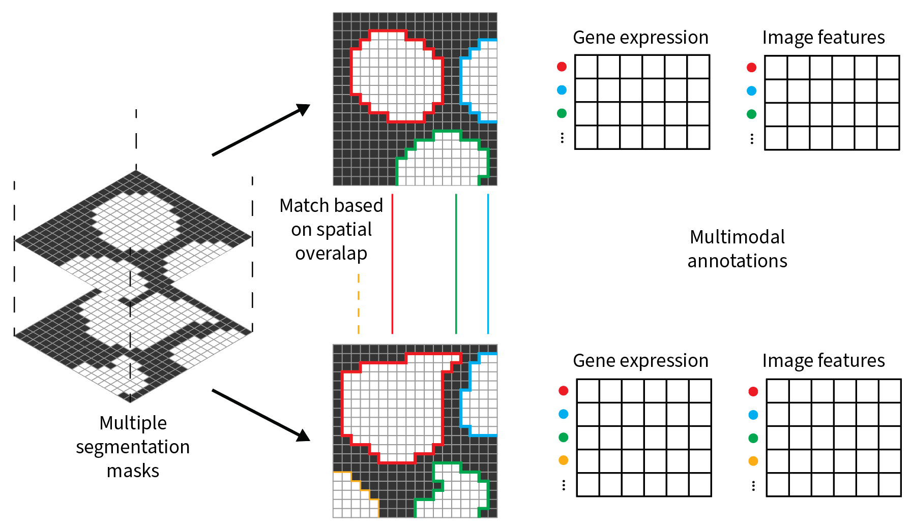
Suppose to have a microscopy image showing cells and to derive two cell segmentation masks from it, using two different algorithms. The segmentation masks may be similar but not identical: some cells may greatly overlap but others may be present in one segmentation but not in the other. Also, you may be interested in storing some annotations for the cells of the two segmentation masks, such as gene expression and image features.

You may want to compare the two segmentation masks based on spatial overlap and match/subset the tables to the common instances. This use case can be addresed using the SOPA, a tool relying on the spatialdata infrastructure.

In particular, the use case described above require the following steps, available in spatialdata and/or in SOPA:

• store the microscopy image and the two segmentation masks (labels objects)

• store the gene expression and image feature information for each of the two segmentation masks

• (implemented in SOPA) convert the segmentation masks to shapes element (GeoDataFrame objects of polygons/multipolygons)

• change the annotation target of the tables from the labels to the newly created shapes elements

• (implemented in SOPA) match the polygonal segmentation masks based on spatial overlap using the geopandas APIs

• filter/match the tables with the new set of common cells using the spatialdata join operations