Transformations and coordinate systems#
In this notebook, we will describe some usage principles for transformations and coordinate systems in spatialdata.SpatialData.
Let’s first import some useful libraries and define a simple function to plot the data downstream.
import math

import matplotlib.pyplot as plt
import spatialdata_plot
from spatialdata.datasets import raccoon
from spatialdata.transformations import (
    Affine,
    Identity,
    MapAxis,
    Scale,
    Sequence,
    Translation,
    get_transformation,
    get_transformation_between_coordinate_systems,
    set_transformation,
)
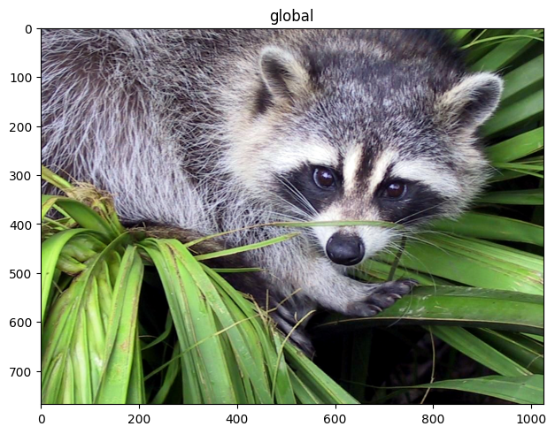
We will use the spatialdata.datasets.raccoon() dummy dataset to showcase the usage of transformations and coordinate systems, that consits of:
an image
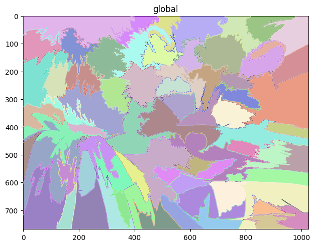
a segmentation mask
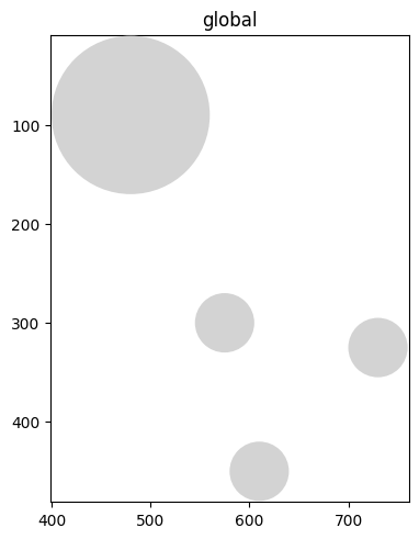
few circles
Let’s inspect the image’s elements
Image#
sdata = raccoon()

print(sdata)

sdata.pl.render_images().pl.show()
INFO     Transposing `data` of type: <class 'dask.array.core.Array'> to ('c', 'y', 'x').
SpatialData object with:
├── Images
│     └── 'raccoon': SpatialImage[cyx] (3, 768, 1024)
├── Labels
│     └── 'segmentation': SpatialImage[yx] (768, 1024)
└── Shapes
      └── 'circles': GeoDataFrame shape: (4, 2) (2D shapes)
with coordinate systems:
▸ 'global', with elements:
        raccoon (Images), segmentation (Labels), circles (Shapes)
Segmentation mask (as labels)#
sdata.pl.render_labels().pl.show()
Circles (as shapes)#
sdata.pl.render_shapes().pl.show()
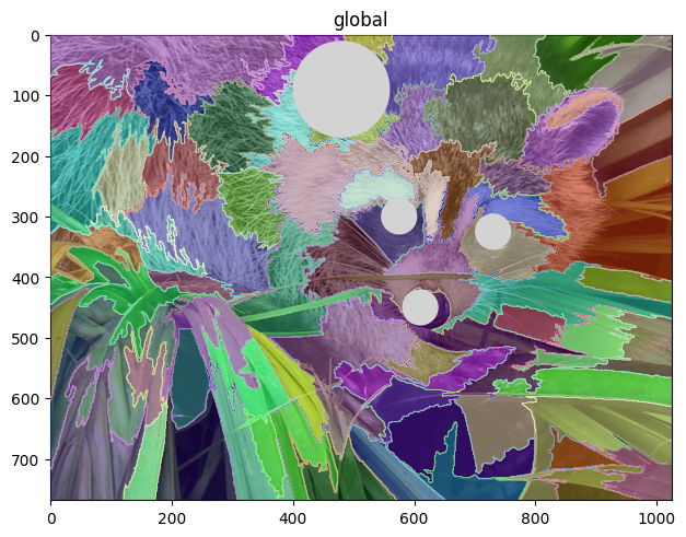
We can either plot these separately or overlay them
fig, axs = plt.subplots(ncols=3, figsize=(12, 3))

sdata.pl.render_images().pl.show(ax=axs[0])
sdata.pl.render_labels().pl.show(ax=axs[1])
sdata.pl.render_shapes().pl.show(ax=axs[2])

sdata.pl.render_images().pl.render_labels().pl.render_shapes().pl.show()

Transformations and coordinate systems#
From the repr printed above, you can already see that the SpatialData object has a coordinate_system attribute, which is a spatialdata.coordinate_systems.CoordinateSystem object.
The coordinate_systems defines the coordinate system of the data, and they store the transformations needed for the element to be converted to the coordinate system.
At the moment, there is coordinate system available: global. In this coordinate system, there are 3 elements:
raccoon: the raccoon image.segmentation: the segmentation mask.circles: the circles.
This is the default coordinate system that is added at the parsing stage, if no other transformation is specified. We can also expect that they are all spatialdata.transformations.Identity transformations.
Let’s print the availale coordinate systems in the SpatialData object and the transformations.
print(sdata.coordinate_systems)
print(
    get_transformation(sdata.images["raccoon"]),
    get_transformation(sdata.labels["segmentation"]),
    get_transformation(sdata.shapes["circles"]),
)
['global']
Identity  Identity  Identity
Now that we understood what is a transformation and what is a coordinate system, let’s see how we can use them.
Let’s start by creating a new transformation, a simple spatialdata.transformations.Scale. This transformation will scale the "x" axis by a factor of 2.
scale = Scale([2.0], axes=("x",))

set_transformation(sdata.images["raccoon"], scale, to_coordinate_system="global")

sdata.pl.render_images().pl.render_labels().pl.render_shapes().pl.show()
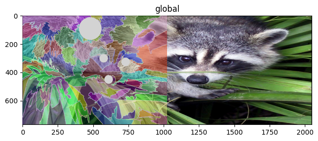
Notice that we passed the elements as is. The transformation API is able to understand what is the type of element as well as how the transformation should be applied to it.
The helper function we defined above does exactly the same thing, but it is a bit more convenient to use.
Various transformations#
Let’s now explore various transformations available in SpatialData.
MapAxis#
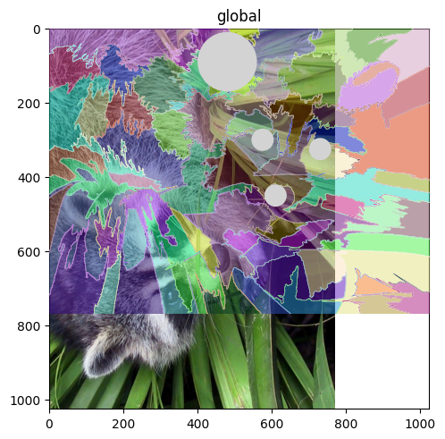
The spatialdata.transformations.MapAxis transformation can be used to permute the axis of the elements.
map_axis = MapAxis({"x": "y", "y": "x"})

set_transformation(sdata.images["raccoon"], map_axis, to_coordinate_system="global")

sdata.pl.render_images().pl.render_labels().pl.render_shapes().pl.show()
Rotation#
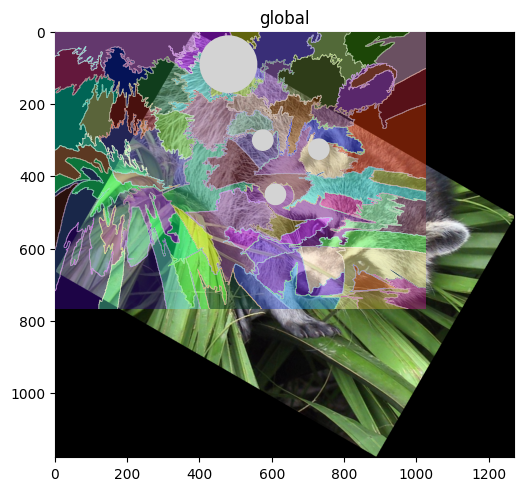
The spatialdata.transformations.Affine transformation can be used to apply an affine transformation to the elements. Let’s start with a rotation.
theta = math.pi / 6
rotation = Affine(
    [
        [math.cos(theta), -math.sin(theta), 0],
        [math.sin(theta), math.cos(theta), 0],
        [0, 0, 1],
    ],
    input_axes=("x", "y"),
    output_axes=("x", "y"),
)

set_transformation(sdata.images["raccoon"], rotation, to_coordinate_system="global")

sdata.pl.render_images().pl.render_labels().pl.render_shapes().pl.show()
Translation#
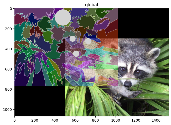
The spatialdata.transformations.Translation transformation can be used to apply a translation to the element.
translation = Translation([500, 300], axes=("x", "y"))

set_transformation(sdata.images["raccoon"], translation, to_coordinate_system="global")

sdata.pl.render_images().pl.render_labels().pl.render_shapes().pl.show()
Affine transformation and composition#
The spatialdata.transformations.Sequence transformation class can be used to compose transformations. This class allows to compose multiple transformations and it can be used even when the axes do not strictly match.
sequence = Sequence([rotation, scale])

set_transformation(sdata.images["raccoon"], sequence, to_coordinate_system="global")

sdata.pl.render_images().pl.render_labels().pl.render_shapes().pl.show()
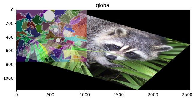
We can also visualize the resulting affine matrix of the transformation.
print(sequence.to_affine_matrix(input_axes=("x", "y"), output_axes=("x", "y")))
[[ 1.73205081 -1.          0.        ]
 [ 0.5         0.8660254   0.        ]
 [ 0.          0.          1.        ]]
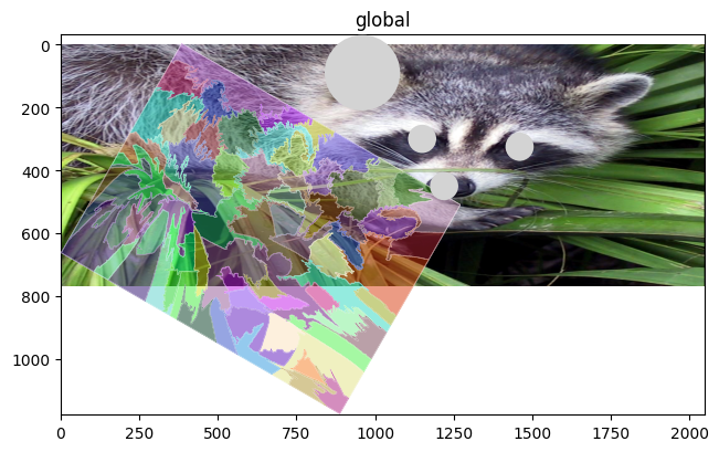
As shown before, transformations can be applied to various elements without the constraint that the axes must match.
For example, a spatialdata.transformations.Scale transformation over axis "x" can be applied both to circles and to images.
set_transformation(sdata.images["raccoon"], scale, to_coordinate_system="global")
set_transformation(sdata.shapes["circles"], scale, to_coordinate_system="global")
set_transformation(sdata.labels["segmentation"], rotation, to_coordinate_system="global")

sdata.pl.render_images().pl.render_labels().pl.render_shapes().pl.show()
WARNING  The transformation matrix is not isotropic, the radius will be scaled by the average of the eigenvalues of
         the affine transformation matrix
Inverse transformations#
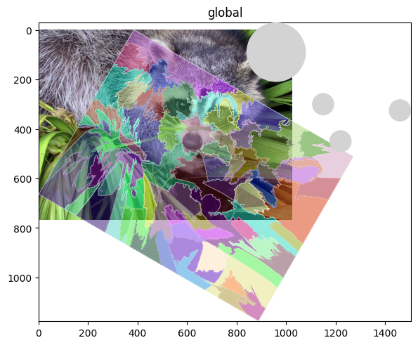
Most of the transformations also have an inverse method that returns the inverse transformation. If composed, they effectively cancel each other out.
sequence = Sequence([rotation, rotation.inverse(), scale, scale.inverse()])

set_transformation(sdata.images["raccoon"], sequence, to_coordinate_system="global")

sdata.pl.render_images().pl.render_labels().pl.render_shapes().pl.show()
WARNING  The transformation matrix is not isotropic, the radius will be scaled by the average of the eigenvalues of
         the affine transformation matrix
Transformations and Axes#
A transformation object can also retrieved the affine matrix with the spatialdata.transformations.Transformation.to_affine_matrix() method.
This method takes as input the axes of the input element and the axes of the output element. The affine matrix is built consistently according to the input and output axes.
Let’s see an example.
print(translation.to_affine_matrix(input_axes=("x", "y"), output_axes=("x", "y")))
print(translation.to_affine_matrix(input_axes=("x", "y", "z"), output_axes=("x", "y", "z")))
[[  1.   0. 500.]
 [  0.   1. 300.]
 [  0.   0.   1.]]
[[  1.   0.   0. 500.]
 [  0.   1.   0. 300.]
 [  0.   0.   1.   0.]
 [  0.   0.   0.   1.]]
The affine matrix is built consistently according to the input and output axes.
The axes at input and output can also have mismatch and the affine matrix will be built accordingly.
print(translation.to_affine_matrix(input_axes=("x", "y", "c"), output_axes=("c", "z", "y", "x")))
[[  0.   0.   1.   0.]
 [  0.   0.   0.   0.]
 [  0.   1.   0. 300.]
 [  1.   0.   0. 500.]
 [  0.   0.   0.   1.]]
notice that z doesn’t appear in the output axes since it was not in the input axes, but c is passed through since it was in the input axes This is the same matrix that gets printed as output above.
x |
y |
c |
||
|---|---|---|---|---|
c |
0 |
0 |
1 |
0 |
z |
0 |
0 |
0 |
0 |
y |
0 |
1 |
0 |
300 |
x |
1 |
0 |
0 |
500 |
0 |
0 |
0 |
1 |
Transformations between coordinate systems#
SpatialData also allows to transform elements between coordinate systems. This is done by using the spatialdata.ops.get_transformation_between_coordinate_systems() function.
The function takes as argument the SpatialData object and the names of the coordinate systems.
It returns the transformation that needs to be applied to the elements in the first coordinate system to be converted to the second coordinate system.
Let’s see an example.
set_transformation(sdata.images["raccoon"], rotation)
print(get_transformation_between_coordinate_systems(sdata, sdata.images["raccoon"], "global"))
print(get_transformation_between_coordinate_systems(sdata, "global", sdata.images["raccoon"]))
Sequence
    Affine (x, y -> x, y)
        [ 0.8660254 -0.5        0.       ]
        [0.5       0.8660254 0.       ]
        [0. 0. 1.]
Sequence
    Affine (x, y -> x, y)
        [0.8660254 0.5       0.       ]
        [-0.5        0.8660254  0.       ]
        [0. 0. 1.]
In the example above, we are effectively only returning the transformation that is needed to convert the elements in the global coordinate system to the global coordinate system (itself).
You can however notice that one transformation is the transpose of the other.
But as mentioned, the function can be used to transform elements between different coordinate systems. Let’s see an example.
We first need to create a new coordinate system for some of the elements. We will just assign an spatialdata.transformations.Identity trasnfomation.
set_transformation(sdata.images["raccoon"], Identity(), "my_other_space0")
set_transformation(sdata.labels["segmentation"], Identity(), "my_other_space1")
print(get_transformation(sdata.images["raccoon"], get_all=True))
print(sdata.coordinate_systems)
{'global': Affine (x, y -> x, y)
    [ 0.8660254 -0.5        0.       ]
    [0.5       0.8660254 0.       ]
    [0. 0. 1.], 'my_other_space0': Identity }
['my_other_space1', 'my_other_space0', 'global']
We then get the transformation between the "global" coordinate system and the "my_other_space0" coordinate system.
As expected, it is a spatialdata.transformations.Sequence transformation with an spatialdata.transformations.Affine and an spatialdata.transformations.Identity composed.
get_transformation_between_coordinate_systems(sdata, "global", "my_other_space0")
Sequence
    Affine (x, y -> x, y)
        [0.8660254 0.5       0.       ]
        [-0.5        0.8660254  0.       ]
        [0. 0. 1.]
    Identity
