Use landmark annotations to align multiple -omics layers#

We will align a Xenium and a Visium datasets for a breast cancer dataset.

We will:

load the data from Zarr;
add landmark annotations to the data using napari;
find an affine similarity transformation that aligns the data.

Loading the data#

You can download the data from here: Xenium dataset, Visium dataset. Please rename the files to xenium.zarr and visium.zarr and place them in the same folder as this notebook (or use symlinks to make the data accessible).

import numpy as np
import spatialdata as sd
from napari_spatialdata import Interactive

xenium_sdata = sd.read_zarr("xenium.zarr")
xenium_sdata

INFO     Instance key `cell_id` could be of type `pd.Categorical`. Consider casting it.                            

SpatialData object with:
├── Images
│     ├── 'morphology_focus': MultiscaleSpatialImage[cyx] (1, 25778, 35416), (1, 12889, 17708), (1, 6444, 8854), (1, 3222, 4427), (1, 1611, 2213)
│     └── 'morphology_mip': MultiscaleSpatialImage[cyx] (1, 25778, 35416), (1, 12889, 17708), (1, 6444, 8854), (1, 3222, 4427), (1, 1611, 2213)
├── Points
│     └── 'transcripts': DataFrame with shape: (42638083, 9) (3D points)
├── Shapes
│     ├── 'cell_boundaries': GeoDataFrame shape: (167780, 1) (2D shapes)
│     ├── 'cell_circles': GeoDataFrame shape: (167780, 2) (2D shapes)
│     ├── 'nucleus_boundaries': GeoDataFrame shape: (167780, 1) (2D shapes)
│     ├── 'visium_landmarks': GeoDataFrame shape: (3, 2) (2D shapes)
│     └── 'xenium_landmarks': GeoDataFrame shape: (3, 2) (2D shapes)
└── Table
      └── AnnData object with n_obs × n_vars = 167780 × 313
    obs: 'cell_id', 'transcript_counts', 'control_probe_counts', 'control_codeword_counts', 'total_counts', 'cell_area', 'nucleus_area', 'region', 'dataset', 'celltype_major', 'celltype_minor'
    var: 'gene_ids', 'feature_types', 'genome'
    uns: 'spatialdata_attrs'
    obsm: 'spatial': AnnData (167780, 313)
with coordinate systems:
▸ 'aligned', with elements:
        morphology_focus (Images), morphology_mip (Images), transcripts (Points), cell_boundaries (Shapes), cell_circles (Shapes), nucleus_boundaries (Shapes)
▸ 'global', with elements:
        morphology_focus (Images), morphology_mip (Images), transcripts (Points), cell_boundaries (Shapes), cell_circles (Shapes), nucleus_boundaries (Shapes), visium_landmarks (Shapes), xenium_landmarks (Shapes)

visium_sdata = sd.read_zarr("visium.zarr")
visium_sdata

SpatialData object with:
├── Images
│     ├── 'CytAssist_FFPE_Human_Breast_Cancer_full_image': MultiscaleSpatialImage[cyx] (3, 21571, 19505), (3, 10785, 9752), (3, 5392, 4876), (3, 2696, 2438), (3, 1348, 1219)
│     ├── 'CytAssist_FFPE_Human_Breast_Cancer_hires_image': SpatialImage[cyx] (3, 2000, 1809)
│     └── 'CytAssist_FFPE_Human_Breast_Cancer_lowres_image': SpatialImage[cyx] (3, 600, 543)
├── Shapes
│     └── 'CytAssist_FFPE_Human_Breast_Cancer': GeoDataFrame shape: (4992, 2) (2D shapes)
└── Table
      └── AnnData object with n_obs × n_vars = 4992 × 18085
    obs: 'in_tissue', 'array_row', 'array_col', 'spot_id', 'region', 'dataset', 'clone'
    var: 'gene_ids', 'feature_types', 'genome'
    uns: 'clone_colors', 'region_colors', 'spatial', 'spatialdata_attrs'
    obsm: 'spatial': AnnData (4992, 18085)
with coordinate systems:
▸ 'aligned', with elements:
        CytAssist_FFPE_Human_Breast_Cancer_full_image (Images), CytAssist_FFPE_Human_Breast_Cancer (Shapes)
▸ 'downscaled_hires', with elements:
        CytAssist_FFPE_Human_Breast_Cancer_hires_image (Images), CytAssist_FFPE_Human_Breast_Cancer (Shapes)
▸ 'downscaled_lowres', with elements:
        CytAssist_FFPE_Human_Breast_Cancer_lowres_image (Images), CytAssist_FFPE_Human_Breast_Cancer (Shapes)
▸ 'global', with elements:
        CytAssist_FFPE_Human_Breast_Cancer_full_image (Images), CytAssist_FFPE_Human_Breast_Cancer (Shapes)

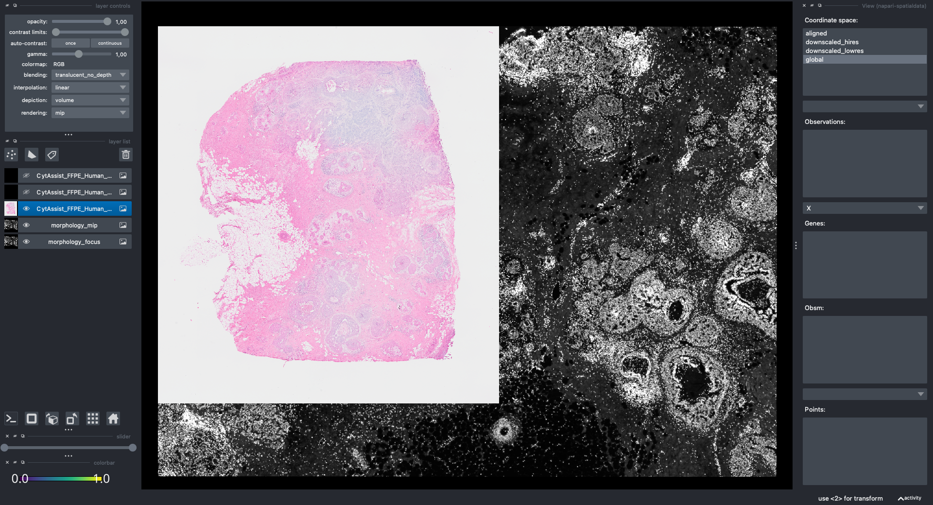
Let’s visualize the data with napari.

Note: we are working with the napari developers to improve performance when visualizing large collections of geometries. For the sake of this example let’s just show the Xenium and Visium images.

Here is a screenshot of the napari viewer. The images are not spatially aligned.

Adding landmark annotations#

Let’s add some landmarks annotations using napari. We will add 3 landmarks to the Visium image to mark recognizable anatomical structures. We will then add, 3 landmarks to the Xenium image to the corresponding anatomical structures, in the same order. One can add more than 3 landmarks per image, as long as the order match between the images.

This is the procedure to annotate and save the landmark locations (shown in the GIF):

open napari with Interactive() from napari_spatialdata
create a new Points layer in napari
(optional) rename the layer
(optional) change the color and points size for easier visualization
click to add the annotation point
(optional) use the napari functions to move/delete points
save the annotation to the SpatialData object by pressing Shift + E (if you called Interactive() passing multiple SpatialData objects, the annotations will be saved to one of them).

For reproducibility, we hardcoded in this notebook the landmark annotations for the Visium and Xenium data. We will add them to the respective SpatialData objects, as if they were were saved with napari.

from spatialdata.models import ShapesModel

visium_landmarks = ShapesModel.parse(
    np.array([[10556.699, 7829.764], [13959.155, 13522.025], [10621.200, 17392.116]]), geometry=0, radius=500
)
visium_sdata.shapes["visium_landmarks"] = visium_landmarks

xenium_landmarks = ShapesModel.parse(
    np.array([[9438.385, 13933.017], [24847.866, 5948.002], [34082.584, 15234.235]]), geometry=0, radius=500
)
xenium_sdata.shapes["xenium_landmarks"] = xenium_landmarks

Finding the affine similarity transformation#

Aligning the images#

We will now use the landmarks to find a similarity affine transformations that maps the Visium image onto the Xenium one.

from spatialdata.transformations import (
    align_elements_using_landmarks,
    get_transformation_between_landmarks,
)

affine = get_transformation_between_landmarks(
    references_coords=xenium_sdata["xenium_landmarks"], moving_coords=visium_sdata["visium_landmarks"]
)
affine

Affine (x, y -> x, y)
    [ 1.61711846e-01  2.58258090e+00 -1.24575040e+04]
    [-2.58258090e+00  1.61711846e-01  3.98647301e+04]
    [0. 0. 1.]

To apply the transformation to the Visium data, we will use the align_elements_using_landmarks function. This function internally calls get_transformation_between_landmarks and adds the transformation to the SpatialData object. It then returns the same affine matrix.

More specifically, we will align the image CytAssist_FFPE_Human_Breast_Cancer_full_image from the Visium data onto the morphology_mip image from the Xenium data. Both images live in the "global" coordinate system (you can see this information by printing xenium_sdata and visium_sdata). The images are not aligned in the "global" coordinate system, and we want them to be aligned in a new coordinate system called "aligned".

affine = align_elements_using_landmarks(
    references_coords=xenium_sdata["xenium_landmarks"],
    moving_coords=visium_sdata["visium_landmarks"],
    reference_element=xenium_sdata["morphology_mip"],
    moving_element=visium_sdata["CytAssist_FFPE_Human_Breast_Cancer_full_image"],
    reference_coordinate_system="global",
    moving_coordinate_system="global",
    new_coordinate_system="aligned",
)
affine

Sequence 
    Identity 
    Affine (x, y -> x, y)
        [ 1.61711846e-01  2.58258090e+00 -1.24575040e+04]
        [-2.58258090e+00  1.61711846e-01  3.98647301e+04]
        [0. 0. 1.]

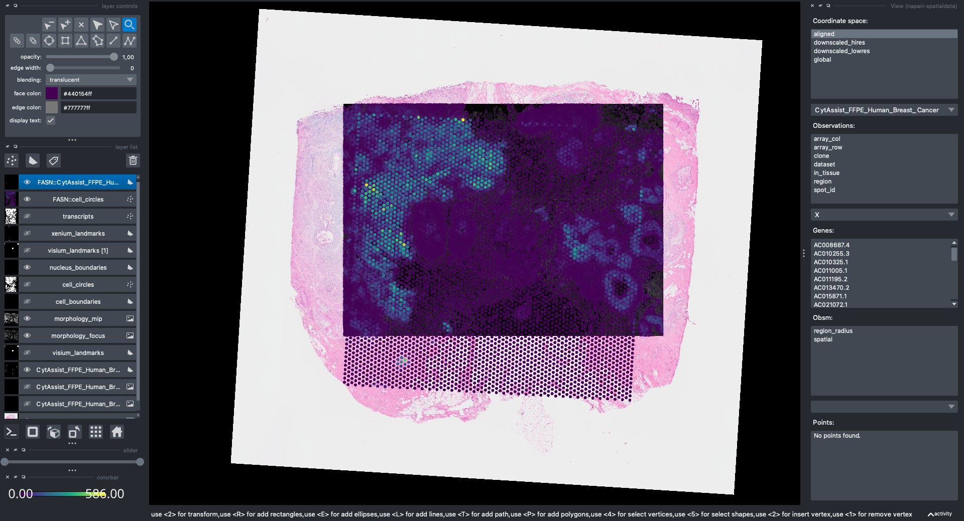
Now the Visium and the Xenium images are aligned in the aligned coordinate system via an affine transformation which rotates, scales and translates the data. We can see this in napari.

Note: the above operation doesn’t modify the data, but it just modifies the alignment metadata which define how elements are positioned inside coordinate system. Both images are mapped to the global coordinate system (in which they are not aligned) and in the aligned coordinate system, where they overlap. In napari you can choose which coordinate system to visualize.

Aligning the rest of the elements#

So far we mapped the Visium image onto the Xenium image in the aligned coordinate system. The rest of the elements are still not aligned. To correct for this we will append the affine transformation calculated above to each transformation for each elements.

Note: this handling of transformation will become more ergonomics in the next code release, removing the need to manually append the transformation as we are doing below. We will update this notebook with the new approach.

from spatialdata import SpatialData
from spatialdata.transformations import (
    BaseTransformation,
    Sequence,
    get_transformation,
    set_transformation,
)


def postpone_transformation(
    sdata: SpatialData,
    transformation: BaseTransformation,
    source_coordinate_system: str,
    target_coordinate_system: str,
):
    for element_type, element_name, element in sdata._gen_elements():
        old_transformations = get_transformation(element, get_all=True)
        if source_coordinate_system in old_transformations:
            old_transformation = old_transformations[source_coordinate_system]
            sequence = Sequence([old_transformation, transformation])
            set_transformation(element, sequence, target_coordinate_system)


postpone_transformation(
    sdata=visium_sdata,
    transformation=affine,
    source_coordinate_system="global",
    target_coordinate_system="aligned",
)

Let’s visualize the result of the alignment with napari.

Saving the alignment back to Zarr#

We will now save the transformations to disk. Notice that this is a lightweight operation because we are just mofiying the objects metadata, not transforming the actual data. This is useful when dealing with large images and when one may need to reiterate multiple steps of landmark-based alignment in order to improve the spatial agreement of the alignment.

from spatialdata import save_transformations

save_transformations(visium_sdata)

Use landmark annotations to align multiple -omics layers

Contents