Squidpy integration

In this notebook, we will describe some usage principles for using SpatialData with squidpy.

Let’s first import some useful libraries and read in a spatialdata dataset.

You might have to install squidpy with !pip install squidpy.

from pathlib import Path

import scanpy as sc
import spatialdata as sd
import spatialdata_plot
import squidpy as sq

We chosed a Xenium dataset formatted in the spatialdata format. You can download the data from here: Xenium dataset. Please rename the file to xenium.zarr and place it in the same folder as this notebook (or use symlinks to make the data accessible).

sdata = sd.read_zarr("xenium.zarr")
sdata

SpatialData object, with associated Zarr store: /Users/macbook/embl/projects/basel/spatialdata-sandbox/xenium_rep1_io/data.zarr
├── Images
│     ├── 'morphology_focus': MultiscaleSpatialImage[cyx] (1, 25778, 35416), (1, 12889, 17708), (1, 6444, 8854), (1, 3222, 4427), (1, 1611, 2213)
│     └── 'morphology_mip': MultiscaleSpatialImage[cyx] (1, 25778, 35416), (1, 12889, 17708), (1, 6444, 8854), (1, 3222, 4427), (1, 1611, 2213)
├── Labels
│     ├── 'cell_labels': MultiscaleSpatialImage[yx] (25778, 35416), (12889, 17708), (6444, 8854), (3222, 4427), (1611, 2213)
│     └── 'nucleus_labels': MultiscaleSpatialImage[yx] (25778, 35416), (12889, 17708), (6444, 8854), (3222, 4427), (1611, 2213)
├── Points
│     └── 'transcripts': DataFrame with shape: (42638083, 8) (3D points)
├── Shapes
│     ├── 'cell_boundaries': GeoDataFrame shape: (167780, 1) (2D shapes)
│     ├── 'cell_circles': GeoDataFrame shape: (167780, 2) (2D shapes)
│     └── 'nucleus_boundaries': GeoDataFrame shape: (167780, 1) (2D shapes)
└── Tables
      └── 'table': AnnData (167780, 313)
with coordinate systems:
    ▸ 'aligned', with elements:
        morphology_mip (Images)
    ▸ 'global', with elements:
        morphology_focus (Images), morphology_mip (Images), cell_labels (Labels), nucleus_labels (Labels), transcripts (Points), cell_boundaries (Shapes), cell_circles (Shapes), nucleus_boundaries (Shapes)

SpatialData has a more complex structure than the (legacy) spatial AnnData format introduced by squidpy. Nevertheless, because it fundamentally uses AnnData as table for annotating regions, with some minor adjustments we can readily use any tool from the scverse ecosystem (squidpy included) to perform downstream analysis.

More precisely, the scverse ecosystem will gradually transition to use SpatialData internally; until that moment the function to_legacy_anndata() from spatialdata_io.experimental can be used to enrich the AnnData in sdata.tables objects to be compatible with the legacy AnnData format.

Generally (i.e. when a single coordinate system is used), the only adjustment required is to populate .obsm['spatial'] with the centroids of the geometries being considered, and this is performed automatically by the spatialdata-io library. For more complex cases, the converter functions to_legacy_anndata() and from_legacy_anndata() can be used (see example at the end of the notebook).

Xenium example

As an example of integration with Squidpy, let’s compute a nearest neighbor graph of the spatial coordiantes of the xenium dataset.

sq.gr.spatial_neighbors(sdata["table"])

After that, we can cluster the cells based on gene expression profiles and compute clustering.

%%time
sc.pp.pca(sdata["table"])
sc.pp.neighbors(sdata["table"])
sc.tl.leiden(sdata["table"])

CPU times: user 1min 39s, sys: 3.31 s, total: 1min 42s
Wall time: 1min 34s

And run the neighbor enrichment analysis in squidpy.

sq.gr.nhood_enrichment(sdata["table"], cluster_key="leiden")
sq.pl.nhood_enrichment(sdata["table"], cluster_key="leiden", figsize=(5, 5))

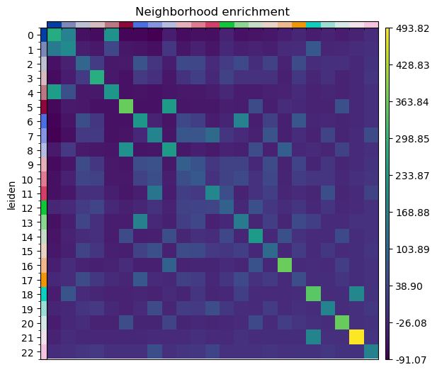
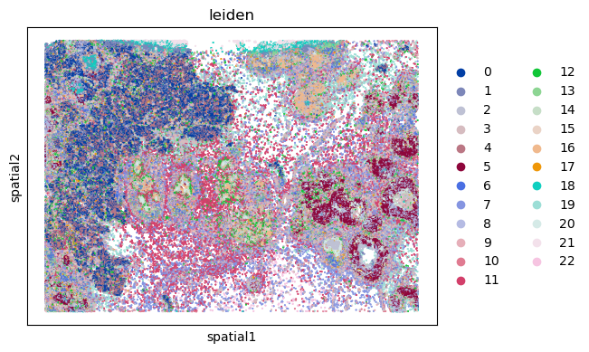
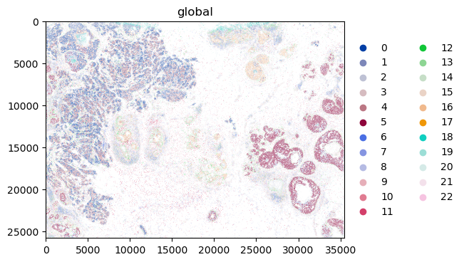
We can finally visualize the results in spatial coordinates both with squidpy as well as with the novel plotting function in spatialdata.

sq.pl.spatial_scatter(sdata["table"], shape=None, color="leiden")

WARNING: Please specify a valid `library_id` or set it permanently in `adata.uns['spatial']`

sdata.pl.render_shapes("cell_circles", color="leiden").pl.show(coordinate_systems="global")

Using the converters from/to the legacy spatial AnnData format

We will now show how to convert from/to the legacy spatialdata AnnData format. The convertes deal with the complexity of having multiple libraries in the legacy format, and with the generality of coordinate systems in SpatialData. For more information please refer to the API documentation of spatialdata-io.

from typing import Literal

import matplotlib.pyplot as plt
import scanpy as sc
import spatialdata_io
import spatialdata_plot
import squidpy as sq
from anndata import AnnData
from spatialdata import SpatialData
from spatialdata._core.query.relational_query import _get_unique_label_values_as_index
from spatialdata.datasets import blobs
from spatialdata.models import TableModel
from spatialdata.transformations import Affine, set_transformation
from spatialdata_io.experimental import from_legacy_anndata, to_legacy_anndata

BlobsTypes = Literal["blobs_labels", "blobs_circles", "blobs_polygons", "blobs_multipolygons"]


def blobs_annotating_element(name: BlobsTypes) -> SpatialData:
    """Returns toy data (blobs) with a table annotating the deised element."""
    sdata = blobs(length=50)
    if name == "blobs_labels":
        instance_id = _get_unique_label_values_as_index(sdata[name]).tolist()
    else:
        instance_id = sdata[name].index.tolist()
    n = len(instance_id)
    new_table = AnnData(shape=(n, 0), obs={"region": [name for _ in range(n)], "instance_id": instance_id})
    new_table = TableModel.parse(new_table, region=name, region_key="region", instance_key="instance_id")
    del sdata.tables["table"]
    sdata["table"] = new_table
    return sdata

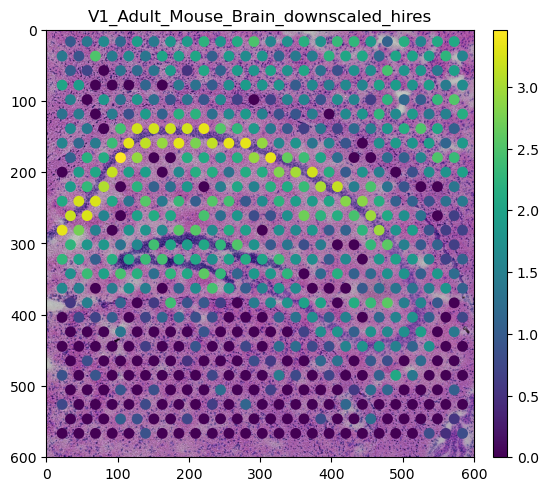
Example of conversion from the legacy AnnData to SpatialData

# some datasets you can play around with
# adata = sq.datasets.visium_fluo_adata()
# adata = sq.datasets.merfish()
adata = sq.datasets.visium_hne_adata_crop()

sdata = from_legacy_anndata(adata)

my_gene = "Itpka"
# broken (multiple table not yet supported in spatialdata-plot), this is being fix in https://github.com/scverse/spatialdata-plot/pull/220
sdata.pl.render_images("V1_Adult_Mouse_Brain_hires_image").pl.render_shapes(color=my_gene).pl.show()
plt.show()

INFO     Transposing `data` of type: <class 'dask.array.core.Array'> to ('c', 'y', 'x').                           
INFO     Transposing `data` of type: <class 'dask.array.core.Array'> to ('c', 'y', 'x').                           
INFO     Dropping coordinate system 'V1_Adult_Mouse_Brain_downscaled_lowres' since it doesn't have relevant        
         elements.                                                                                                 

Example of conversion from SpatialData to the legacy AnnData, showing also that affine transformations are handled

element = "blobs_circles"
sdata = blobs_annotating_element(element)
image = "blobs_multiscale_image"

affine = Affine([[1, 2, 3], [-2, 1, 6], [0, 0, 1]], input_axes=("x", "y"), output_axes=("x", "y"))
set_transformation(sdata[element], affine, "transformed")
set_transformation(sdata[image], affine, "transformed")

adata = to_legacy_anndata(sdata, include_images=True, coordinate_system="transformed")

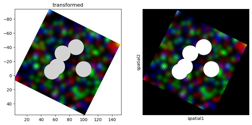
axes = plt.subplots(1, 2, figsize=(10, 5))[1]
sdata.pl.render_images(image).pl.render_shapes(element).pl.show(coordinate_systems=["transformed"], ax=axes[0])
sc.pl.spatial(
    adata,
    spot_size=300,
    library_id=image,
    img_key="hires",
    na_color="white",
    show=True,
    crop_coord=(0, 2000, 0, 2000),
    ax=axes[1],
)